Recruiting-Kanban & Experiment Dashboard (ATS Pipeline, Power BI)

The dashboard represents the recruiting process in Kanban logic. Important key figures such as Work-in-Process (WIP), Cycle Time, Throughput, Conversion, and Time-to-Hire change daily or weekly. Therefore, this case is well suited to make agile control visible. The report layout follows the ideas of IBCS/SUCCESS: a clear statement in the title, uniform colors, and a reduced design so that HR, IT, and hiring managers use a common data language

Data Basis and ETL

The solution uses three synthetic CSV files. ats_pipeline_events contains the event log per candidate and stage (Applied, Screen, Interview, Offer, Hired/Rejected) with stage_start_date and stage_end_date as well as contextual fields such as Department, Role, Seniority, Location, Source, Recruiter, and Variation (A/B). ats_candidates provides master data on the candidate (e.g., applied_date, recruiter, variation). ats_requisitions describes the vacancy (req_id, department, role, location, seniority). In Power BI, the files are imported, data types are set (especially the date fields), empty strings are treated as null, and identifiers are standardized. This event log is the appropriate foundation for Kanban because start and end timestamps per stage later directly enable calculations for CFD, Cycle Time, Aging, and Throughput.

Data Model (Star Schema)

The model follows a star schema. The fact table ats_pipeline_events lies at the center. The dimensions ats_candidates, ats_requisitions, Dim_Date, and Dim_Stage provide the axes of analysis. Between Dim_Date[Date] and events[stage_start_date] there is an active 1:n relationship for “Flow-in.” Additionally, an inactive relationship from Dim_Date[Date] to events[stage_end_date] is stored. This inactive connection is deliberately activated in measures using USERELATIONSHIP() in order to correctly control “Flow-out” (e.g., hires per week). Attributes that appear twice in the fact table (e.g., department) are hidden in the report; for analyses, the columns from the dimensions are used. The model is lean and can easily be extended in sprints.

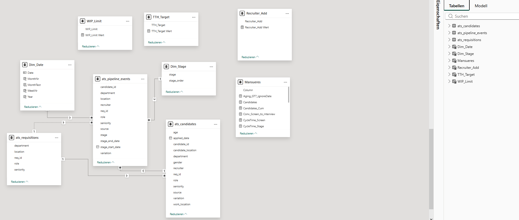
Dimensions and Sorting

Dim_Date is generated from the minimum of the start date and the maximum of the end date and is extended by Year, MonthNr, MonthText, and WeekNr. MonthText is sorted by MonthNr, and the table is marked as a date table. Dim_Stage defines the order of stages via stage_order (Applied … Rejected), so that diagrams sort consistently. These two tables ensure a clean time and process logic throughout the entire report.

Key Figures and Analytical Logic (DAX)

The key figures combine descriptive transparency with simple prescriptive signals. Three central measures are presented as examples.Time-to-Hire (average in days) and Gap-to-Target. First, the average duration between “Applied” and “Hired” is calculated. Afterwards, it is compared with a target value set via a What-If parameter.

TTH :=
VAR AppliedDate =
CALCULATE(
MIN(ats_pipeline_events[stage_start_date]),
ALLEXCEPT(ats_pipeline_events, ats_pipeline_events[candidate_id]),
ats_pipeline_events[stage] = "Applied")
VAR HiredDate :=
CALCULATE(
MAX(ats_pipeline_events[stage_end_date]),
ALLEXCEPT(ats_pipeline_events, ats_pipeline_events[candidate_id]),
ats_pipeline_events[stage] = "Hired")
RETURN
AVERAGEX(
VALUES(ats_pipeline_events[candidate_id]),
DATEDIFF(AppliedDate, HiredDate, DAY)
)

The target value is created as a What-If parameter TTH_Target; the gap results as Gap_TTH = [TTH] − [TTH_Target Value]. A positive gap indicates an SLA deviation and provides a clear impulse for action.

WIP Limit and Over-Limit. Kanban actively controls the number of parallel cases. WIP counts candidates in the active stages. With a second What-If parameter WIP_Limit, the limit is set; Over-Limit immediately signals bottlenecks.

WIP :=
CALCULATE(
DISTINCTCOUNT(ats_pipeline_events[candidate_id]),
ats_pipeline_events[stage] IN {"Applied","Screen","Interview","Offer"})
WIP_Over_Limit :=
VAR Over = [WIP] - [WIP_Limit Wert]
RETURN IF(Over > 0, Over, 0)
If Over-Limit > 0, overload is present. In practice, this leads to a measure, for example lowering the limit or increasing capacity.

Throughput per Week (Flow-out). For Hires and Rejections, the report counts cases by end date. For this purpose, the inactive date relationship is deliberately activated per measure.

Hires_Woche :=
CALCULATE(
DISTINCTCOUNT(ats_pipeline_events[candidate_id]),
ats_pipeline_events[stage] = "Hired",
USERELATIONSHIP(Dim_Date[Date], ats_pipeline_events[stage_end_date]))

Rejected_Woche :=
CALCULATE(
DISTINCTCOUNT(ats_pipeline_events[candidate_id]),
ats_pipeline_events[stage] = "Rejected",
USERELATIONSHIP(Dim_Date[Date], ats_pipeline_events[stage_end_date]))

The time series makes the outflow visible and shows whether the process delivers steadily or fluctuates. Together with the Screen-Interview conversion and the Cycle Time per stage, clear indications of bottlenecks emerge.

Report Design and Visualization

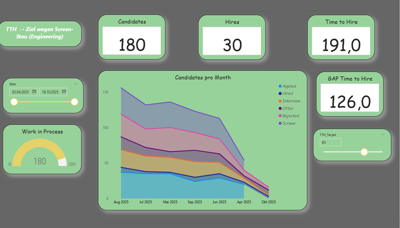
The first report page provides a compact overview: five KPI cards (Candidates, Hires, WIP, TTH, Gap_TTH) show status and target achievement. A gauge compares WIP with the limit and marks overload. The Cumulative Flow Diagram (stacked area chart) represents the flow across months; in-process stages are shown in shades of blue, Hired in green, Rejected in red. A SAY title names the core message, for example “TTH above target due to backlog in Screen (Engineering).”

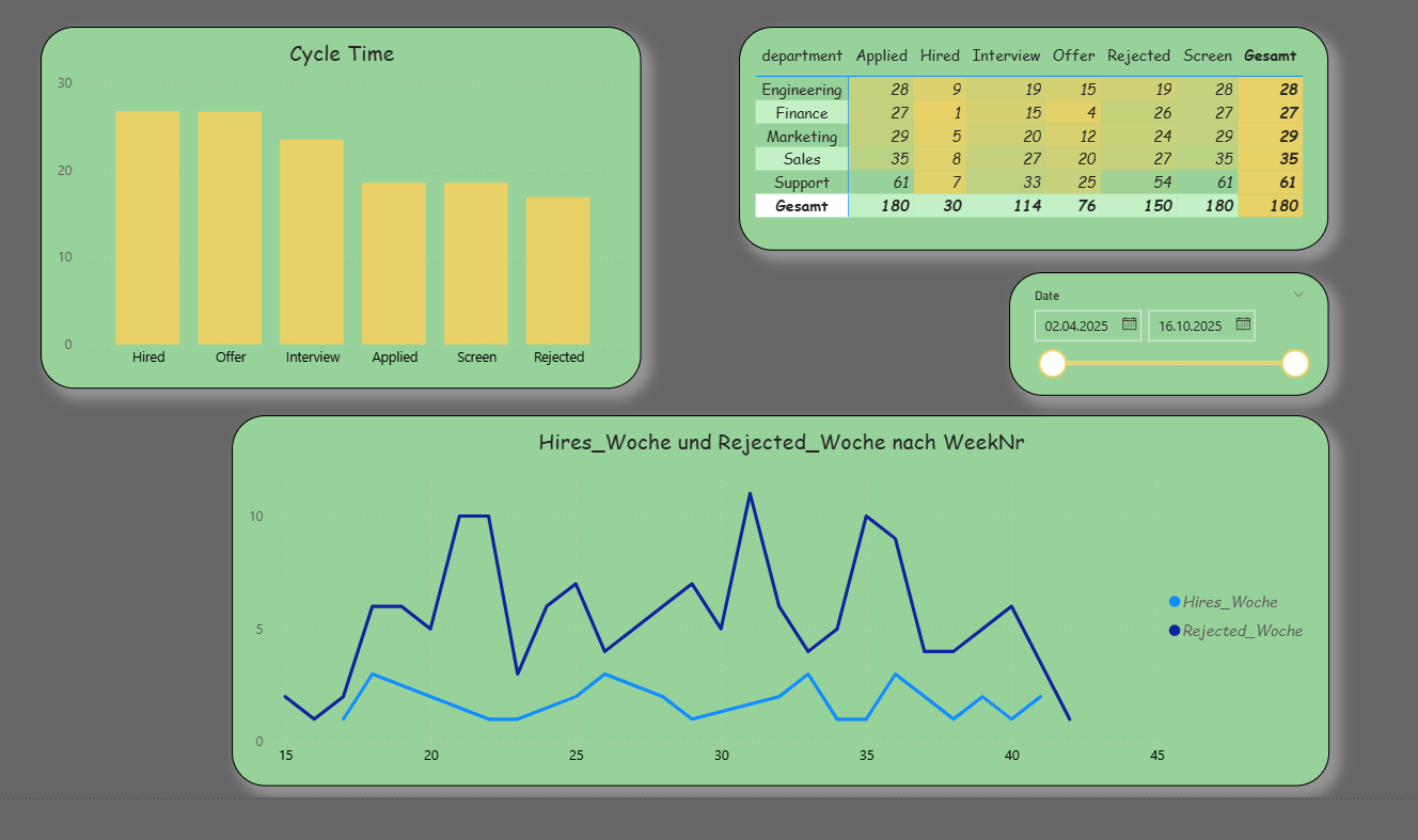
The second report page serves root cause analysis. The Cycle Time per stage shows where most time is lost. A matrix with Department × Stage highlights the distribution of starts per stage; this count based on the start date is robust and responds cleanly to date filters. In addition, Hires_Week and Rejected_Week are displayed as lines to examine the outflow over the weeks.

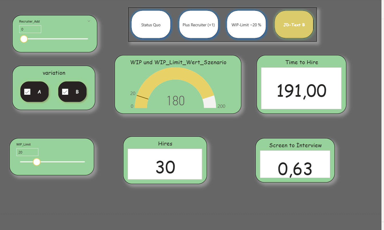
The third report page supports decisions through scenarios. What-If parameters (WIP_Limit, TTH_Target, optional Recruiter_Add) and bookmarks (Status Quo, Plus Recruiter, WIP Limit −20%, JD Text B) change the view with one click. The KPI cards, the gauge, and a small “Over-Limit” card respond immediately. Optionally, a simple rule can output a recommendation, for example: If Over-Limit > 0 and Cycle Time in “Screen” is high, then lower the limit or deploy +1 recruiter; if conversion is low, test variation B.

Agile Value and Types of Analysis

The solution combines descriptive transparency with prescriptive indications. Descriptively, KPI cards, CFD, Cycle Time, and Throughput provide a clear picture of the current state and bottlenecks. Simple predictive indications arise from trends in Throughput and Conversion. Prescriptively, Gap-to-Target, WIP Limit, and the scenarios take effect: they directly lead to concrete measures within the process. Through the IBCS-oriented design, communication across departments remains consistent and understandable.